Getting started#
Welcome to the absolute beginner’s guide to py-fatigue! If you have comments or suggestions, please don’t hesitate to file an issue or make a pull request on our GitHub repo: https://github.com/OWI-Lab/py_fatigue/.
Welcome to py-fatigue!#
py-fatigue was originally part of the DYNAwind suite of tools for wind turbine structural health monitoring and analysis. The tool has been detached from the project and now relies on the following PyPi packages only:
Python ([3.8, 3.9, 3.10] for v1.*.*, [3.10, 3.11, 3.12, 3.13] for v2.*.*, 64-bit only)
numpy
plotly
pandas
numba vers. ^0.57 (for v1.*.*), vers. ^0.61 (for v2.*.*)
matplotlib
pydantic
The package bundles the main functionality for performing cyclic stress (fatigue and crack growth) analysis and cycle-counting.
Installing py-fatigue#
py-fatigue is freely available on GitHub and gets maintained through CI/CD phylosophy. The package requires Python 3.8 or higher, and it requires a 64-bit version of Python.
To install the toolbox from PyPI, simply run:
pip install py-fatigue
and you will get the latest published version.
How to import py-fatigue#
To access py-fatigue and its functions import it in your Python code like this:
import py_fatigue as pf
How to use py-fatigue#
The main functionality of py-fatigue is to perform cyclic stress analysis and cycle counting. The toolbox provides a number of functions to perform these tasks. The main functions are:
cycle_count: collects all the functions related with cycle-counting fatigue data and allows a simpler representation of a rainflow-counted stress vs. time history.
material: allows the definition of some fatigue-specific material properties such as
SN curve and
geometry: enables the instantiation of specific crack geometries for crack propagation analysis, i.e.
Infinite surface.
Hollow cylinder with a crack on its external surface.
damage: the module collecting the fatigue life calculation models.
stress-life: fatigue analysis based on the cycle-counting and SN curve.
crack_growth: crack propagation (growth) analysis based on the cycle-counting, the Paris’ law and the geometrical definition of a crack case (defect geometry and medium).
mean_stress: a module to calculate the mean stress correction factor for the cycle-counting.
testing: a module to simulate different kinds of load histories. The most generic type of load history can be simulated using the get_sampled_time and get_random_data functions, as shown in the example below.
Example#
In the following example, starting from a randomly generated signal, we will:
calculate the rainflow
export the cycle-count matrix
reconstruct the CycleCount object from the exported matrix
define the SN curve
calculate the Palmgren-Miner damage
define the Paris’ law
define a crack geometry
run a crack growth analysis.
The damage and crack growth analyses will be also executed by means of the pandas DataFrame accessors that py-fatigue implements.
Random signal simulation#
import py_fatigue as pf
import py_fatigue.testing as test
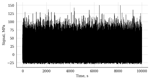
# Simulate a random signal
t = test.get_sampled_time(duration=10000, fs=10)
s = test.get_random_data(
t=t, min_=-30, range_=180, random_type="weibull", a=2., seed=42
)
# Plot the signal
plt.plot(t, s, 'k', lw=0.5)
plt.xlabel("Time, s")
plt.ylabel("Signal, MPa")
plt.show()
Cycle-count definition#
# CycleCount definition
cycle_count = pf.CycleCount.from_timeseries(
    time=t, data=s, mean_bin_width=3., range_bin_width=3.,
)
cycle_count
Cycle counting object |
Random signal |
|---|---|
largest full stress range, MPa |
179.026964 |
largest stress range, MPa |
180.0 |
number of full cycles |
33317 |
number of residuals |
23 |
number of small cycles |
0 |
stress concentration factor |
N/A |
residuals resolved |
False |
mean stress-corrected |
No |
Cycle-count matrix#
# Exporting the cycle-count matrix in the legacy format, i.e. not
# accounting for mean stresses. This function has been kept for
# backwards compatibility.
exp_dict_legacy = cycle_count.as_dict(
    max_consecutive_zeros=20, damage_tolerance_for_binning=0.2, legacy=True
)
print(exp_dict_legacy)
{"nr_small_cycles": 99, "range_bin_lower_bound": 0.2, "range_bin_width": 3.0,
 "hist": [1346.0, 1485.0, 1433.0, 1397.0, 1455.0, 1493.0, 1479.0, 1471.0, 1348.0,
          1432.0, 1361.0, 1234.0, 1236.0, 1203.0, 1146.0, 1103.0, 1072.0,  983.0,
           957.0,  853.0,  808.0,  806.0,  679.0,  659.0,  570.0,  520.0,  449.0,
           451.0,  397.0,  376.0,  289.0,  259.0,  236.0,  237.0,  164.0,  160.0,
           120.0,   89.0,   85.0,   92.0,   60.0,   54.0,   39.0,   20.0,   24.0,
            24.0,   17.0,   12.0,   10.0,    8.0,    2.0,    5.0,    6.0,    1.0,
             0.0,    2.0,    0.0,    1.0,    0.0,    1.0], "lg_c": [],
 "res": [ 64.9527,  76.1706,  83.8523, 112.9550, 115.8100, 123.7286, 125.4990,
         137.6065, 138.7786, 139.5674, 140.8493, 159.0391, 159.1209, 167.0853,
         167.1570, 180.0000, 179.8804, 122.3010, 115.1474,  58.9131,  53.7620,
          31.8885],
 "res_sig": [ 49.8674, -15.0853,  61.0853, -22.7670,  90.1880, -25.6220,  98.1066,
             -27.3924, 110.2141, -28.5645, 111.0029, -29.8464, 129.1926, -29.9283,
             137.157,  -30.0000, 150.0000, -29.8804,  92.4207, -22.7267,  36.1864,
             -17.5756, 14.3128, 14.2784]}
# Exporting the cycle-count matrix
exp_dict = cycle_count.as_dict(
    max_consecutive_zeros=20, damage_tolerance_for_binning=1
)
print(exp_dict)
{"nr_small_cycles": 99, "range_bin_lower_bound": 0.2, "range_bin_width": 3.0,
 "mean_bin_lower_bound": -25.5, "mean_bin_width": 3.0,
 "hist": [[ 0.0,  1.0],
          [ 1.0,  1.0],
          [ 4.0,  5.0,  4.0,  1.0,  3.0],
          [14.0, 17.0,  9.0, 10.0,  6.0,  4.0,  0.0,  2.0,  1.0],
          [31.0, 31.0, 21.0, 20.0, 13.0, 10.0,  6.0,  7.0,  4.0,  5.0],
          [33.0, 51.0, 24.0, 39.0, 31.0, 28.0, 22.0, 15.0, 13.0,  6.0,  2.0,  3.0,
           1.0],
          [56.0, 68.0, 63.0, 40.0, 45.0, 40.0, 36.0, 41.0, 19.0, 22.0, 18.0, 11.0,
            7.0,  2.0,  1.0],
          [74.0, 91.0, 78.0, 60.0, 78.0, 60.0, 75.0, 46.0, 44.0, 44.0, 40.0, 20.0,
           19.0, 18.0,  4.0,  2.0],
          ...,
          [ 0.0,  2.0,  0.0,  1.0,  0.0,  0.0,  0.0,  0.0,  1.0,  0.0,  0.0,  0.0,
            1.0,  0.0,  0.0,  0.0,  1.0],
          [ 0.0,  0.0,  0.0,  0.0,  0.0,  0.0,  1.0,  0.0,  0.0,  0.0,  0.0,  0.0,
            0.0,  0.0,  0.0,  0.0,  1.0],
          [0.0,  0.0,  0.0,  0.0,  1.0]],
 "lg_c": [[ 52.7204, 157.4858], [ 52.7330, 165.3195], [ 53.0368, 165.7063],
          [ 56.1889, 172.3578], [ 59.9228, 179.0270]],
 "res": [[  17.3910,  64.9527], [ 23.0000,  76.1706], [19.1591,  83.8523],
         [  33.7105, 112.9550], [ 32.2830, 115.8100], [36.2423, 123.7286],
         [  35.3571, 125.4990], [ 41.4109, 137.6065], [40.8248, 138.7786],
         [  41.2192, 139.5674], [ 40.5782, 140.8493], [49.6731, 159.0391],
         [  49.6322, 159.1209], [ 53.6143, 167.0853], [53.5785, 167.1570],
         [  60.0000, 180.0000], [ 60.0598, 179.8804], [31.2702, 122.3010],
         [  34.8470, 115.1474], [  6.7298,  58.9131], [ 9.3054,  53.7620],
         [  -1.6314, 31.8885]],
 "res_sig": [ 49.8674, -15.0853,  61.0853, -22.7670,  90.1880, -25.6220,  98.1066,
             -27.3924, 110.2141, -28.5645, 111.0029, -29.8464, 129.1926, -29.9283,
             137.1570, -30.0000, 150.0000, -29.8804, 92.4207,  -22.7267,  36.1864,
             -17.5756, 14.3128, 14.2784]}
# Reconstructing the CycleCount instance from the exported matrix
cycle_count_d = pf.CycleCount.from_rainflow(exp_dict, name="Random Signal")
cycle_count_d
Cycle counting object |
Random Signal |
|---|---|
largest full stress range, MPa |
179.027 |
largest stress range, MPa |
180.0 |
number of full cycles |
33219 |
number of residuals |
22 |
number of small cycles |
99 |
stress concentration factor |
N/A |
residuals resolved |
False |
mean stress-corrected |
No |
import matplotlib as mpl
import matplotlib.pyplot as plt
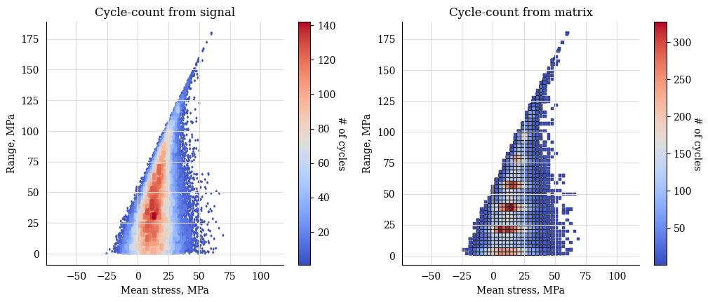
fig, axs = plt.subplots(1, 2, figsize=(12, 4.5))
cycle_count.plot_histogram(fig=fig, ax=axs[0], plot_type="mean-range",
marker="d", s=2, cmap=plt.get_cmap("coolwarm"))
axs[0].set_title("Cycle-count from signal")
cycle_count_d.plot_histogram(fig=fig, ax=axs[1], plot_type="mean-range",
marker="s", s=10, edgecolors="#222",
cmap=plt.get_cmap("coolwarm"), linewidth=0.25)
axs[1].set_title("Cycle-count from matrix")
plt.show()
Stress-Life#
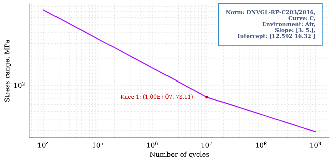
SN Curve definition#
c_air = pf.SNCurve(
    [3, 5],
    intercept=[12.592, 16.320],
    norm="DNVGL-RP-C203/2016",
    environment='Air',
    curve='C'
)
c_air
Damage calculation analysis#
# Calculate damage for the cycle-count objects
damage = pf.damage.stress_life.get_pm(cycle_count=cycle_count, sn_curve=c_air)
damage_d = pf.damage.stress_life.get_pm(cycle_count=cycle_count_d, sn_curve=c_air)
print(f"damage from signal: {sum(damage)}")
print(f"damage from matrix: {sum(damage_d)}")
damage from signal: 0.0013318803351252439
damage from matrix: 0.0013321255571107358
Crack growth#
A crack growth simulation necessitates of three ingredients (objects):
Cycle-counted stress history
Crack growth curve (e.g. Paris’ law)
Crack geometry
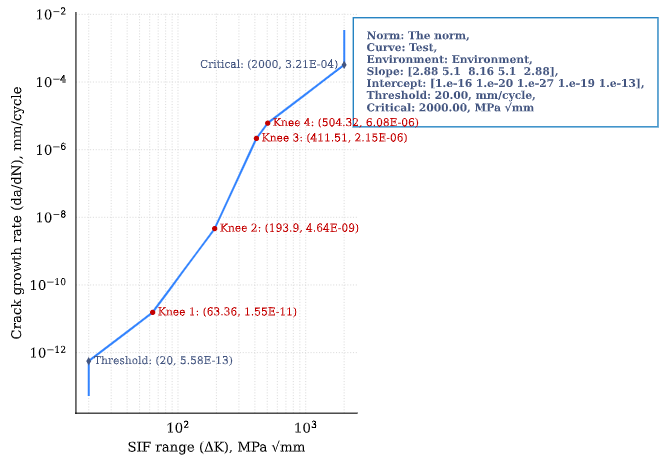
Paris’ curve definition#
SIF = np.linspace(1,2500, 300)
SLOPE = np.array([2.88, 5.1, 8.16, 5.1, 2.88])
INTER = np.array([1E-16, 1E-20, 1E-27, 1E-19, 1E-13])
THRESHOLD = 20
CRITICAL = 2000
pc = pf.ParisCurve(slope=SLOPE, intercept=INTER, threshold=THRESHOLD,
                   critical=CRITICAL, norm="The norm",
                   environment="Environment", curve="nr.")
pc
Crack geometry definition#
geo = pf.geometry.HollowCylinder(
  initial_depth=5.,
  thickness=10.,
  height=30.,
  outer_diameter=30.,
  crack_position="external"
)
geo
HollowCylinder(
  _id=HOL_CYL_01,
  initial_depth=5.0,
  outer_diameter=300.0,
  thickness=10.0,
  height=30.0,
  crack_position=external,
)
Crack growth analysis#
cg = pf.damage.crack_growth.get_crack_growth(
  cycle_count, pc, geo, express_mode=True
)
print(f"Cycles to end: {int(cg.final_cycles)}")
Fatigue spectrum applied w/o failure. Stopping calculation
Cycles to end: 3328
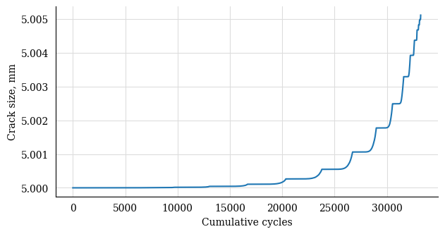
cg_d = pf.damage.crack_growth.get_crack_growth(
  cycle_count_d, pc, geo, express_mode=True
)
print(f"Cycles to end: {int(cg.final_cycles)}")
Fatigue spectrum applied w/o failure. Stopping calculation
Cycles to end: 3320
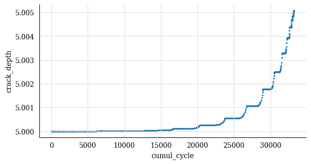
plt.plot(np.cumsum(cg_d.count_cycle), cg_d.crack_depth)
plt.xlabel("Cumulative cycles")
plt.ylabel("Crack size, mm")
plt.show()
Working with pandas DataFrames#
It’s possible to translate the CycleCount object to a pandas DataFrame and use
the implemented accessors py_fatigue.damage.stress_life.PalmgrenMiner
(miner) and py_fatigue.damage.crack_growth.CrackGrowth (cg) to
perform the stress-life and propagation analyses as shown above.
import pandas as pd

df = cycle_count.to_df()

# Stress-life
df.miner.damage(sn_curve=c_air)
# Crack-growth
df.cg.calc_growth(cg_curve=pc, crack_geometry=geo)
df.miner.plot_histogram()
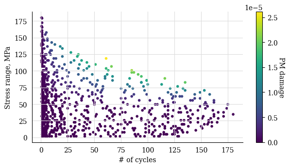
df.plot(kind="scatter", x="cumul_cycle", y="crack_depth", s=2)