4. CycleCount definition#
The CycleCount class incorporates the main information about a processed signal for fatigue analysis.
a. Constant fatigue load#
Note
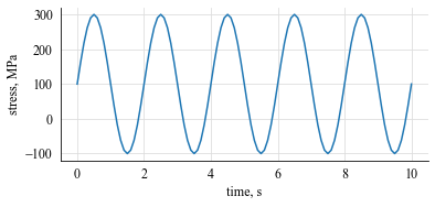
In this example we define a fatigue stress signal in the form of a sinusoidal function.
We then feed our signal to the CycleCount class.
Define the time and stress arrays
t = np.arange(0, 10.1, 0.1)  # (in seconds)
s = 200 * np.sin(np.pi*t) + 100   # (in MPa)
plt.plot(t, s)
plt.xlabel("time, s")
plt.ylabel("stress, MPa")
plt.show()
Define the CycleCount instance
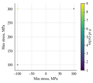
cc = pf.CycleCount.from_timeseries(s, t, name="Example")
cc
Example |
|
|---|---|
Cycle counting object |
|
largest full stress range, MPa, |
None |
largest stress range, MPa |
400.0 |
number of full cycles |
0 |
number of residuals |
11 |
number of small cycles |
0 |
stress concentration factor |
N/A |
residuals resolved |
False |
mean stress-corrected |
No |
fig, ax = plt.subplots(1,1, figsize=(4.5, 4))
cc.plot_histogram(fig=fig)
Showing the exported dictionary
cc.as_dict(legacy_expoprt=True)
Gives:
{
    'nr_small_cycles': 0,
    'range_bin_lower_bound': 0.2,
    'range_bin_width': 0.05,
    'hist': [],
    'lg_c': [],
    'res': [200.0, 400.0, 400.0, 400.0, 400.0, 400.0,
            400.0, 400.0, 400.0, 400.0, 200.0],
    'res_sig': [100.0, 300.0, -100.0, 300.0, -100.0, 300.0,
               -100.0, 300.0, -100.0, 300.0, -100.0, 100.0]
}
b. Weibull-distributed signal#
Note
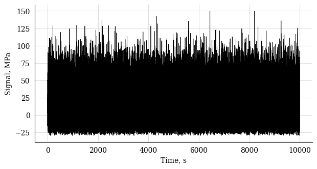
In this example we define a Weibull-distributed fatigue stress signal.
CycleCount class.
Define the time and stress arrays
import py_fatigue.testing as test

# Simulate a random signal
t = test.get_sampled_time(duration=10000, fs=10)
s = test.get_random_data(
  t=t, min_=-30, range_=180, random_type="weibull", a=2., seed=42
)
# Plot the signal
plt.plot(t, s, 'k', lw=0.5)
plt.xlabel("Time, s")
plt.ylabel("Signal, MPa")
plt.show()
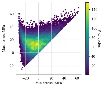
Define the CycleCount instance
  # CycleCount definition
cycle_count = pf.CycleCount.from_timeseries(
  time=t, data=s, mean_bin_width=3., range_bin_width=3.,
)
cycle_count
Cycle counting object |
Random signal |
||||||||
|---|---|---|---|---|---|---|---|---|---|
largest full stress range, MPa |
179.026964 |
||||||||
largest stress range, MPa |
180.0 |
||||||||
number of full cycles |
33317 |
||||||||
number of residuals |
23 |
||||||||
number of small cycles |
0 |
||||||||
stress concentration factor |
N/A |
||||||||
residuals resolved |
False |
||||||||
mean stress-corrected |
No |
fig, ax = plt.subplots(1,1, figsize=(4.5, 4))
cc.plot_histogram(fig=fig)
Exporting the rainflow counted signal as a json dictionary, both in legacy (no mean stress) and new format.
# Exporting the cycle-count matrix in the legacy format, i.e. not
# accounting for mean stresses. This function has been kept for
# backwards compatibility.
exp_dict_legacy = cycle_count.as_dict(
    max_consecutive_zeros=20, damage_tolerance_for_binning=0.2, legacy=True
)
print(exp_dict_legacy)
{"nr_small_cycles": 99, "range_bin_lower_bound": 0.2, "range_bin_width": 3.0,
 "hist": [1346.0, 1485.0, 1433.0, 1397.0, 1455.0, 1493.0, 1479.0, 1471.0, 1348.0,
          1432.0, 1361.0, 1234.0, 1236.0, 1203.0, 1146.0, 1103.0, 1072.0,  983.0,
           957.0,  853.0,  808.0,  806.0,  679.0,  659.0,  570.0,  520.0,  449.0,
           451.0,  397.0,  376.0,  289.0,  259.0,  236.0,  237.0,  164.0,  160.0,
           120.0,   89.0,   85.0,   92.0,   60.0,   54.0,   39.0,   20.0,   24.0,
            24.0,   17.0,   12.0,   10.0,    8.0,    2.0,    5.0,    6.0,    1.0,
             0.0,    2.0,    0.0,    1.0,    0.0,    1.0], "lg_c": [],
 "res": [ 64.9527,  76.1706,  83.8523, 112.9550, 115.8100, 123.7286, 125.4990,
         137.6065, 138.7786, 139.5674, 140.8493, 159.0391, 159.1209, 167.0853,
         167.1570, 180.0000, 179.8804, 122.3010, 115.1474,  58.9131,  53.7620,
          31.8885],
 "res_sig": [ 49.8674, -15.0853,  61.0853, -22.7670,  90.1880, -25.6220,  98.1066,
             -27.3924, 110.2141, -28.5645, 111.0029, -29.8464, 129.1926, -29.9283,
             137.157,  -30.0000, 150.0000, -29.8804,  92.4207, -22.7267,  36.1864,
             -17.5756, 14.3128, 14.2784]}
# Exporting the cycle-count matrix
exp_dict = cycle_count.as_dict(
    max_consecutive_zeros=20, damage_tolerance_for_binning=1
)
print(exp_dict)
{"nr_small_cycles": 99, "range_bin_lower_bound": 0.2, "range_bin_width": 3.0,
 "mean_bin_lower_bound": -25.5, "mean_bin_width": 3.0,
 "hist": [[ 0.0,  1.0],
          [ 1.0,  1.0],
          [ 4.0,  5.0,  4.0,  1.0,  3.0],
          [14.0, 17.0,  9.0, 10.0,  6.0,  4.0,  0.0,  2.0,  1.0],
          [31.0, 31.0, 21.0, 20.0, 13.0, 10.0,  6.0,  7.0,  4.0,  5.0],
          [33.0, 51.0, 24.0, 39.0, 31.0, 28.0, 22.0, 15.0, 13.0,  6.0,  2.0,  3.0,
           1.0],
          [56.0, 68.0, 63.0, 40.0, 45.0, 40.0, 36.0, 41.0, 19.0, 22.0, 18.0, 11.0,
            7.0,  2.0,  1.0],
          [74.0, 91.0, 78.0, 60.0, 78.0, 60.0, 75.0, 46.0, 44.0, 44.0, 40.0, 20.0,
           19.0, 18.0,  4.0,  2.0],
          ...,
          [ 0.0,  2.0,  0.0,  1.0,  0.0,  0.0,  0.0,  0.0,  1.0,  0.0,  0.0,  0.0,
            1.0,  0.0,  0.0,  0.0,  1.0],
          [ 0.0,  0.0,  0.0,  0.0,  0.0,  0.0,  1.0,  0.0,  0.0,  0.0,  0.0,  0.0,
            0.0,  0.0,  0.0,  0.0,  1.0],
          [0.0,  0.0,  0.0,  0.0,  1.0]],
 "lg_c": [[ 52.7204, 157.4858], [ 52.7330, 165.3195], [ 53.0368, 165.7063],
          [ 56.1889, 172.3578], [ 59.9228, 179.0270]],
 "res": [[  17.3910,  64.9527], [ 23.0000,  76.1706], [19.1591,  83.8523],
         [  33.7105, 112.9550], [ 32.2830, 115.8100], [36.2423, 123.7286],
         [  35.3571, 125.4990], [ 41.4109, 137.6065], [40.8248, 138.7786],
         [  41.2192, 139.5674], [ 40.5782, 140.8493], [49.6731, 159.0391],
         [  49.6322, 159.1209], [ 53.6143, 167.0853], [53.5785, 167.1570],
         [  60.0000, 180.0000], [ 60.0598, 179.8804], [31.2702, 122.3010],
         [  34.8470, 115.1474], [  6.7298,  58.9131], [ 9.3054,  53.7620],
         [  -1.6314, 31.8885]],
 "res_sig": [ 49.8674, -15.0853,  61.0853, -22.7670,  90.1880, -25.6220,  98.1066,
             -27.3924, 110.2141, -28.5645, 111.0029, -29.8464, 129.1926, -29.9283,
             137.1570, -30.0000, 150.0000, -29.8804, 92.4207,  -22.7267,  36.1864,
             -17.5756, 14.3128, 14.2784]}
It is also possible defining the CycleCount instance from the exported CycleCount dictionary (json file).
# Reconstructing the CycleCount instance from the exported matrix
cycle_count_d = pf.CycleCount.from_rainflow(exp_dict, name="Random Signal")
cycle_count_d
Cycle counting object |
Random Signal |
||||||||
|---|---|---|---|---|---|---|---|---|---|
largest full stress range, MPa |
179.027 |
||||||||
largest stress range, MPa |
180.0 |
||||||||
number of full cycles |
33219 |
||||||||
number of residuals |
22 |
||||||||
number of small cycles |
99 |
||||||||
stress concentration factor |
N/A |
||||||||
residuals resolved |
False |
||||||||
mean stress-corrected |
No |
A slightly more complicated plot to show the Markov matrix as well as the cumulative (or non-cumulative) rainflow matric both for cc and cc_dct:
fig, axs = plt.subplots(2,2, figsize=(13, 10))
cc.plot_histogram(fig=fig, ax=axs[0][0], plot_type="mean-range")
cc_dct.plot_histogram(fig=fig, ax=axs[0][1], plot_type="mean-range")
cc.plot_histogram(fig=fig, ax=axs[1][0], plot_type="counts-range-cumsum", s=30)
cc_dct.plot_histogram(fig=fig, ax=axs[1][1], plot_type="counts-range",
                      marker='s', s=20,
                      cmap=plt.get_cmap("gnuplot2"))  # chg cmap
axs[1][1].set_xscale("log")
axs[1][0].set_xscale("log")
plt.show()
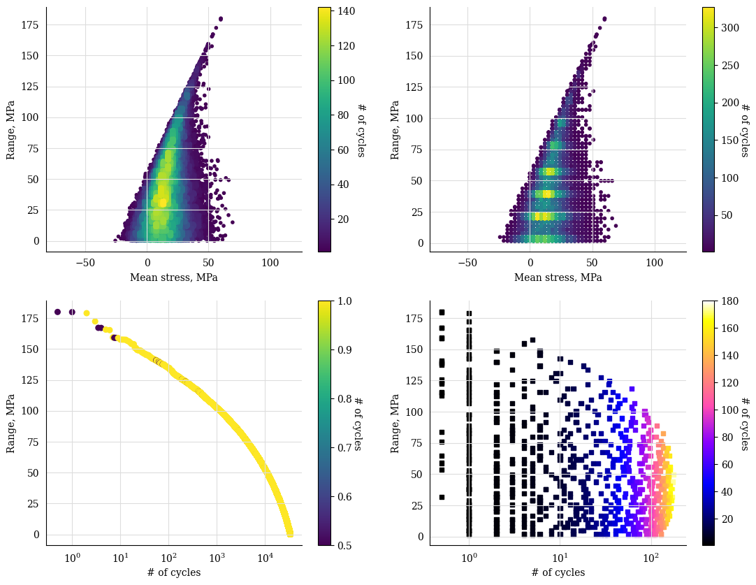
Comparison of histograms built from signal and from its cycle-count matrix#