7. Stress-Life damage calculation#
This section contains some examples of damage calculations using the stress-life approach.
The module py_fatigue.damage.stress_life contains all the
damage models related to the stress-life approach.
The simplest and most common damage model is the
Palmgren-Miner (py_fatigue.damage.stress_life.calc_pm,
py_fatigue.damage.stress_life.get_pm) model.
Besides the linear damage accumulation rule, py-fatigue also
provides a series of nonlinear damage accumulation models callable through
py_fatigue.damage.stress_life.calc_nonlinear_damage and
py_fatigue.damage.stress_life.get_nonlinear_damage
Manson and Halford
Si Jian et al.
Pavlou
Leve
The generic form of a nonlinear damage rule is:
where \(n_j\) is the number of cycles in the fatigue histogram at the \(j\)-th cycle, \(N_j\) is the number of cycles to failure at the \(j\)-th cycle, \(e_{j, j+1}\) is the exponent for the \(j\)-th and \(j+1\)-th cycles, \(M\) is the number of load blocks in the fatigue spectrum.
The formula is conveniently rewritten as pseudocode:
# retrieve N_j using the fatigue histogram and SN curve
# retrieve the exponents e_{j, j+1}
#  calculate the damage
D = 0
for j in range(1, M+1):
    D = (D + n_j / N_j) ^ e_{j, j+1}
Specifically, for the damage models currently implemented in py_fatigue, the exponents are:
Manson and Halford: \(e_{j, j+1} = \left(\frac{N_{j}}{N_{j+1}}\right)^{\alpha}\) with \(\alpha=0.4\) usually.
Si Jian et al.: \(e_{j, j+1} = \sigma_{j+1} / \sigma_{j}\) where \(\sigma_{j+1}\) is the stress amplitude for the \(j\)-th cycle.
Pavlou: \(e_{j, j+1} = \left(\frac{\Delta \sigma_j / 2}{\sigma_U}\right)^{\alpha}\) where \(\Delta \sigma_j/2\) is the stress amplitude, \(\sigma_U\) is the ultimate stress, \(\Delta \sigma\) is the stress range and \(\alpha=0.75\) (usually) is the exponent.
Leve: \(e_{j, j+1} =\text{constant}\).
1. Palmgren-Miner#
a. Constant fatigue load (sinoid)#
Note
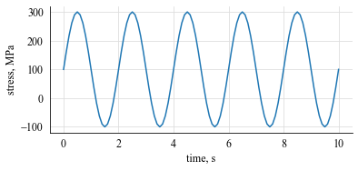
In this example we define a fatigue stress signal in the form of a sinusoidal function and calculate the damage using the Palmgren-Miner Rule.
We then feed our signal to the CycleCount class.
Define the time and stress arrays
t = np.arange(0, 10.1, 0.1)  # (in seconds)
s = 200 * np.sin(np.pi*t) + 100   # (in MPa)
plt.plot(t, s)
plt.xlabel("time, s")
plt.ylabel("stress, MPa")
plt.show()

Define the CycleCount instance
cc = pf.CycleCount.from_timeseries(s, t, name="Example")
cc
Example |
|
|---|---|
Cycle counting object |
|
largest full stress range, MPa, |
None |
largest stress range, MPa |
400.0 |
number of full cycles |
0 |
number of residuals |
11 |
number of small cycles |
0 |
stress concentration factor |
N/A |
residuals resolved |
False |
mean stress-corrected |
No |
Define the SN curve
1w3a = pf.SNCurve([3, 5], [10.970, 13.617],
2                 norm='DNVGL-RP-C203', curve='W3', environment='Air')
There are two main ways of calculating the damage from cc.
Using the
get_pm()method.Converting cc to a
DataFrameand using the dataframe extension calleddf.miner.damage().
1df = cc.to_df()
2df.miner.damage(w3a)
3print(df)
4print(f"Damage from pandas df: {df['pm_damage'].sum()}")
5print(f"Damage from  function: {pf.damage.stress_life.get_pm(cc, w3a)}")
Which outputs:
index |
count_cycle |
mean_stress |
stress_range |
cycles_to_failure |
pm_damage |
|---|---|---|---|---|---|
0 |
0.5 |
200 |
200 |
11665.68 |
0.000043 |
1 |
0.5 |
100 |
400 |
1458.21 |
0.000343 |
2 |
0.5 |
100 |
400 |
1458.21 |
0.000343 |
3 |
0.5 |
100 |
400 |
1458.21 |
0.000343 |
4 |
0.5 |
100 |
400 |
1458.21 |
0.000343 |
5 |
0.5 |
100 |
400 |
1458.21 |
0.000343 |
6 |
0.5 |
100 |
400 |
1458.21 |
0.000343 |
7 |
0.5 |
100 |
400 |
1458.21 |
0.000343 |
8 |
0.5 |
100 |
400 |
1458.21 |
0.000343 |
9 |
0.5 |
100 |
400 |
1458.21 |
0.000343 |
10 |
0.5 |
0 |
200 |
11665.68 |
0.000043 |
Damage from pandas df: 0.0031716971435032985
Damage from  function: 0.0031716971435032985
