5. CycleCount sum

a. List of signals (timeseries)

Note

In this example we define a list of segmented timeseries and compare the sum of the CycleCount from segmented data with the CycleCount from concatenated data.

We then apply the solve_lffd() method, as per LFFD to recover the effect of low-frequency cycles.

Define the time and stress arrays

# input data
from collections import defaultdict
import py_fatigue.testing as test

signal_duration = int(86400 / 60)  # (in minutes)
max_peak = 200  # (in MPa)

# list of timestamps
timestamps = []

# list of timeseries
timeseries = []

# concatenated time and stress arrays
conc_time = np.empty(0)
conc_stress = np.empty(0)

# main loop
for i in range(0,30):
  np.random.seed(i)
  print(f"{i+1} / 30", end = "\r")
  min_ = - np.random.randint(3, 40)
  range_ = np.random.randint(1, 200)
  timestamps.append(
      datetime.datetime(2020, 1, i + 1, tzinfo=datetime.timezone.utc)
  )
  timeseries.append(defaultdict())

  time = test.get_sampled_time(duration=signal_duration, fs=10, start=i)
  stress = test.get_random_data(
    t=time, min_=min_, range_=range_, random_type="weibull", a=2., seed=i
  )
  conc_time = np.hstack(
    [conc_time, time + conc_time[-1] if len(conc_time) > 0 else time]
  )
  conc_stress = np.hstack([conc_stress, stress])
  timeseries[i]["data"] = stress
  timeseries[i]["time"] = time
  timeseries[i]["timestamp"] = timestamps[-1]
  timeseries[i]["name"] = "Example sum"

# Generating the timeseries dictionary
timeseries.append({"data": conc_stress, "time": conc_time,
                   "timestamp": timestamps[0], "name": "Concatenated"})

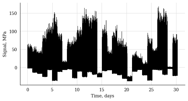
# concatenated timeseries plot
plt.plot(conc_time/60/24, conc_stress, 'k', lw=0.5)
plt.xlabel("Time, s")
plt.ylabel("Signal, MPa")
plt.show()

Define the CycleCount instances

cc = []
for t_s in timeseries:
    cc.append(pf.CycleCount.from_timeseries(**t_s))

# sum of the CycleCount instances
cc_sum = cc[0] + cc[1]

# CyclCeCount from concatenated data
cc_conc = pf.CycleCount.from_timeseries(**timeseries[-1])

CycleCount from concatenated timeeries

	Concatenated
Cycle counting object
largest full stress range, MPa,	189.71765
largest stress range, MPa	206.0
number of full cycles	143860
number of residuals	31
number of small cycles	0
stress concentration factor	N/A
residuals resolved	False
mean stress-corrected	No

# sum of the CycleCount instances
cc_sum.solve_lffd()

CycleCount from summed segmented timeeries after LFFD recovery

	Example sum
Cycle counting object
largest full stress range, MPa,	189.71765
largest stress range, MPa	206
number of full cycles	143860
number of residuals	31
number of small cycles	0
stress concentration factor	N/A
residuals resolved	True
mean stress-corrected	No

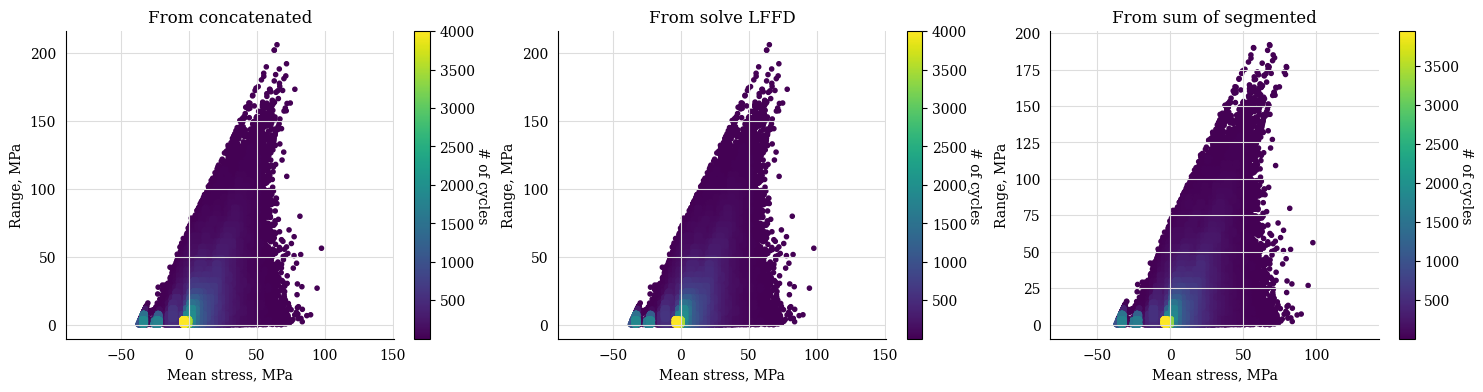
fig, axs = plt.subplots(1, 3, figsize=(16, 4))
cc_conc.plot_histogram(fig=fig, ax=axs[0], plot_type="mean-range")
cc_sum.solve_lffd().plot_histogram(fig=fig, ax=axs[1], plot_type="mean-range")
cc_sum.plot_histogram(fig=fig, ax=axs[2], plot_type="mean-range")

plt.show()

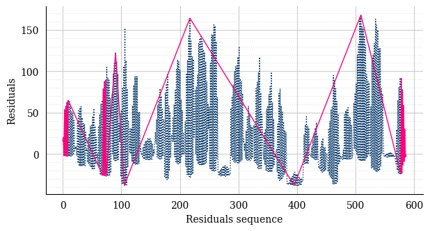
cc_sum.plot_half_cycles_sequence(lw=1)
plt.show()